Necessity or Luxury
questions to O. Kochukhov, G. Wade & D. Shulyak

03.2.2012   Extensive tests ?

  02.2.2012   Disappearing observations and codes archived forever ?

  01.2.2012   Strong enough to influence the line profiles ?

  31.1.2012   Exciting times ?

  30.1.2012   Magic in the air ?

  29.1.2012   Largely irrelevant assertions ?

  28.1.2012   An unusually high contrast ?

  27.1.2012   Serious problems with an "untested" inversion code ?

  26.1.2012   A profoundly multi-line, multi-phase character ?

  25.1.2012   A more natural way ?

  24.1.2012   An artefact of limited computational capabilities ?

  23.1.2012   A significant and fertile research direction ?

  22.1.2012   Magnetic or non-magnetic abundance DI analyses ?

  21.1.2012   Systematic application of reasoning ?

  20.1.2012   Published in conference proceedings ?

  19.1.2012   More precise line opacities ?

  18.1.2012   Exotic languages ?

A) 18.1.2012

"... without a recourse to the next generation computers or exotic
programming languages advocated by S12."

Are the authors aware of the fact that very recent statistics on the
popularity of programming languages show that Ada is in 17th place
whereas Fortran is relegated to the 27th place?

Are the authors aware that their very lives depends on the power and
reliability of Ada each time they take a plane, be it Airbus or Boeing?

       http://www.adaic.org/advantages/projects/


B) 19.1.2012

"The resulting sampling at ∼10^6 frequency points yields more precise
line opacities than the ATLAS12 calculations at 120 000 frequencies
employed in the study by S12."

Can the authors provide any plot that would prove that the effects on
the temperature gradient changes radically (or even noticeably) with
the increase from 120000 points to 1 million points?

Would the differences in line profile as a function of metallicity as
shown in Fig. 3 of S12 change in any (substantial) way?

"Our computation of the line absorption coefficient was based
on the atomic data for ∼6.6 × 10^7 lines extracted from the VALD
data base (Kupka et al. 1999). In addition to the standard lists of
transitions between measured energy levels, this includes a new
massive predicted line list calculated by R. Kurucz and discussed
by Grupp, Kurucz & Tan (2009)."

"The lower panel in Fig. 2 illustrates the depth dependence of
temperature for the same set of LLMODELS atmospheres as mentioned
above, but now as a function of tau_R. It is obvious that the effects
of different iron abundance introduce much smaller changes
compared to those implied by the T vs. tau_5000 plot."

Extra lines mean extra opacity and line blanketing. Shouldn't the
effects as shown in Figs. 1 and 2 of S12 be enhanced? How large is
this effect?

What then is the point in insisting that the metallicity effects on
the atmospheric structure are much smaller than those claimed by S12
when plotted against tau_R?

"A complete analysis should always include not only comparisons of
the depth-dependent thermodynamic properties, but also different
spectroscopic and photometric observables (such as energy distributions,
hydrogen lines, photometric parameters, metallic line spectra) in order
to quantify the importance of detected changes in the context of
particular investigations."

Aren't energy distributions in the context of this particular
investigations presented in Fig. 2 of S12, isn't the effect on
hydrogen lines plotted in Fig. 5, aren't metallic line spectra
shown in Figs. 3, 4, and 6?


C) 20.1.2012

"One of the most outstanding is the large chemical abundance contrasts
in atmospheres of Ap stars, which according to DI analyses can be quite
extreme (e.g. variations of several orders of magnitude across the
stellar surface). In regions of high enrichment, some metals are
sometimes inferred to be only a factor of ∼30 less abundant compared
to hydrogen (e.g.,Kuschnig et al. 1998), which is challenging to explain
theoretically."

"The choice by S12 of the abundance DI studies yielding “unrealistic”
elemental overabundances is highly selective, confined to two extreme
results, both published in conference proceedings (Kuschnig et al.
1998; Piskunov et al. 1998). This ignores the majority of DI studies
published in the refereed literature which reported much more modest
abundance contrasts."

Could it be that these 2 paragraphs are slightly inconsistent? Why
are the results from exactly the same paper initially presented as
a "challenge" for theoreticians, 12 pages and many arguments later
as "published in conference proceedings" ?

What is wrong in calling results where Cr is more abundant than
hydrogen "unrealistic"? And what is wrong in not calling "modest
abundance contrasts" unrealistic?

How do we have to understand the statement that the latter have been
"published in the refereed literature" whereas the former were
"published in conference proceedings"? Isn't it unthinkable that
any scientist should try to publish irreproducible and/or barely
credible results in proceedings?

Wouldn't the findings of Piskunov et al. (1988) constitute a much
more challenging task for theoreticians than those by Kuschnig et al.
(1998)? Wouldn't it be incredibly exciting to try to guess at the
physics of such an extreme part of the stellar atmosphere, to figure
out what kind of mechanism (as yet unknown) could lead to such a
prominent chromium spot of non-negligible extension on kappa Psc.
How would such an extreme star evolve with time? Can you imagine
anything more gratifying for the best people in the field of stellar
structure and stellar atmospheres than to model this unique object?


D) 21.1.2012

"A reader may also note that with systematic application of the
reasoning of S12, one is bound to conclude that stellar surface
mapping is completely unfeasible with photometric data – a ludicrous
assertion given the well-known success of many photometric star spot
investigations (e.g., Korhonen, Berdyugina & Tuominen 2002; Lanza et
al. 2009; Mosser et al. 2009; Lüftinger et al. 2010a). For instance,
the high photometric stability of the CoRoT satellite allowed Mosser
et al. (2009) to detect photometric signatures of spots as small as
a few degrees across, whereas according to S12 such a study should
not have provided any surface spatial resolution at all."

How comes it that the authors of that paragraph think it appropriate
to apply reasoning valid for spectra with moderate phase coverage
(watch the gaps), S/N ratio between 240 and 1020, a resolving power
of 35000 - and just 6 lines used for magnetic imaging - to photometric
star spot investigations? Why should it constitute a "systematic
application of the reasoning of S12" to pretend that the information
on the magnetic fine structure contained in at most 100 wavelength
points for each of the Stokes QUV parameters is equivalent to the
information on the extension of intensity spots provided by thousands
or even tens of thousands of observations with micro-mag accuracy,
perfect phase coverage, and with high to extreme time resolution?


E) 22.1.2012

"A similar magnetic inversion technique, employing a general spherical
spherical harmonic expansion, was independently developed by Donati
(2001) and successfully used for the Stokes IV ZDI of global fields
of Ap stars (Lüftinger et al. 2010a), ..."

Isn't it clearly stated in Lüftinger et al. (2010a) that for the
magnetic inversion, the Stokes V profiles have been calculated under
the assumption, valid in the weak field limit, that Stokes V is
proportional to ..... and dI/dlam the wavelength derivative of the
local Stokes I line profile. We further assume that there are no
large-scale brightness or abundance inhomogeneities over the stellar
surface, so that synthetic Stokes I profiles are locally the same over
the whole photosphere"?

Would it be frivolous to ask how this approach can possibly be
reconciled with the existence of 4 bright photometric spots shown in
their Fig. 4 ?

Do Lüftinger et al. (2010a) not clearly state that they do not carry
out ZDI but only DI ? "By applying the Doppler imaging technique (DI),
we are able to translate the partially very pronounced variations in
the spectral line profiles of HD50773, linked to stellar rotation, into
surface maps of the abundance distribution. The longitude of a spot is
directly deduced from the wavelength position of the distortion within
the profile, whereas its latitude can only be derived from time-series
observations."

Isn't this confirmed by the authors themselves? "Non-magnetic abundance
DI analyses (Kochukhov et al. 2004b; Lüftinger et al. 2010a) as well
as MDI studies based on the Stokes I and V spectra (Kochukhov et al.
2002; Lüftinger et al. 2010b) normally avoid such strong lines, dealing
with weak or intermediate strength features."


F) 23.1.2012

"Contrary to the impression conveyed by S12, this prominent influence
of chemical composition on the structure of stellar surface layers is
well-known to the Ap star community and has been addressed in numerous
applications of the LLMODELS code to individual stars (Kochukhov et al.
2009b; Shulyak, Kochukhov & Khan 2008; Shulyak et al. 2009, 2010b;
Lüftinger et al. 2010a) – a significant and fertile research direction,
seemingly unnoticed by S12."

"We assume that there are no ... abundance inhomogeneities over the
stellar surface". Does this not mean that Lüftinger et al. (2010a) have
neglected even the most basic effects of metallicity on the profiles?
Did they not treat Stokes profiles in the spots exactly like those outside?

Did we not restrict our statement on the neglect of differential line
blanketing to the Doppler mapping community: "Notwithstanding the
ground-breaking work of Chandrasekhar (1935), differential line
blanketing – between spot and photosphere – in stellar atmospheres has
never been taken into account by Doppler mapping experts."?

Did we not prove well aware of a "fertile research direction" by stating:
"Especially for recent work, this seems a bit strange since Khan & Shulyak
(2007) have shown the nonnegligible effects of Fe and Cr overabundances
on stellar atmospheres and on abundance estimates."?

Where in the papers cited above is there any mention of metallicity-
dependent local atmospheres to be used in Doppler mapping? Do Kochukhov
et al. (2009b) not rather assume "homogeneously distributed abundances"
as a basis for stratification modelling?


G) 24.1.2012

"Finally, S12 state that the large overabundances inferred from
DI are at odds with the predictions of theoretical diffusion calculations,
which have not been shown to produce such large accumulations.
In fact, both cited theoretical diffusion studies have artificially
limited the maximum accumulation of chemical elements to
log(Nel/Ntot) = −2.3 (LeBlanc et al. 2009) or log(Nel/Ntot) =
−3.0 (Alecian & Stift 2007) in order to avoid numerical instabilities.
However, in both studies this limit has been reached for
certain chemical elements at some optical depths (see Fig. 3 of
Alecian & Stift (2007) and Fig. 4 of LeBlanc et al. (2009)). Thus,
the lack of very high elemental overabundances in the equilibrium
diffusion calculations is an artefact of the limited computational
capabilities of the currently used atomic diffusion codes.

Is it possible that the authors are not aware of the fact that the
limit to the accumulation of elements has to be imposed because otherwise
the physical approximations would break down? Why then do the authors
impute the "lack of very high elemental overabundances" to the "limited
computational capabilities" of the codes? Does this speculation not
simply show that the authors are not acquainted with the basic physics
implemented in these codes and well described in the relevant literature?

Is it not true that the copious literature known to us - and kindly
provided in a truly concise form by courtesy of the authors - leaves
no doubt as to the fact that all Doppler mapping results obtained so
far are based on models with vertically constant abundances? Does this
not imply that the extreme Cr, Fe or Si abundances have to be extreme
from the bottom to the top of the atmosphere? Is it on the other hand
not true that Fig. 3 in Alecian & Stift (2007) clearly shows that
extreme abundances of Mg, Si, Ca, and Fe are never found in layers
below log tau_5000 = -1, and that for Fe the abundances are even below
solar in the upper layers, unless there is a very strong horizontal
field?

So how could the authors ever meaningfully compare (Z)DI results based
on vertically constant extreme abundances (still using mean atmospheres
based on moderate metal abundances) with extreme abundances found only
over a restricted interval in optical depth?


H) 25.1.2012

"A more natural way to compare model atmosphere structures is to plot
physical quantities against an optical depth computed with some mean
opacity coefficient. In particular, an optical depth based on the
Rosseland opacity coefficient kappa_R has a certain advantage: spectral
regions with the smallest opacities transfer most of the radiative
energy and at the same time contribute most to kappa_R. Examining the
physical quantities of different models as a function of tau_R allows
one to trace changes of the model structure on a natural depth scale
representing frequency-integrated properties of the radiation field."

What is so "natural" about the tau_R scale in the context of spectral
line synthesis, polarised or not? Doesn't each and every textbook on
radiative transfer and line formation teach us that we are dealing
with a problem requiring monochromatic opacities, monochromatic optical
depths? When KW10 synthese the Fe II line at 5018.440 used in magnetic
inversions, do they not require the continuous opacity at this wavelength
and do they not carry out a straight addition of continuous and line
opacity? When one is interested in the effect of the change in
atmospheric structure on this iron line, is it not more natural to
use the tau_5000 scale (a wavelength so close to this line!!) than to
employ a harmonic mean taken from the far UV to the far infrared?


I) 26.1.2012

"But this profoundly multi-line, multi-phase character of modern
MDI was not considered by S12, who limited their analysis to a
single spectral line at one rotational phase."

Wasn't it clearly said in the S12 paper that at the phases for
which the signal of a small high-contrast magnetic spot was plotted
"the respective signals due to the spot are largest"? So where is
the alleged analysis of a single spectral line at a single rotational
phase? Isn't it quite legitimate to illustrate a point by showing
the maximum effect to be expected?

By the way, where do we find the "profoundly multi-line,
multi-phase character of modern MDI" in the analysis of 53 Cam?
Remember that Kochukhov et al. (2004) state unequivocally:
"Secondly, the amplitude of the disk-integrated Stokes Q and U
line profiles of 53 Cam is very low and a conspicuous linear
polarization signal can be detected in only a few strong
magnetically-sensitive spectral lines at a limited number of
rotational phases (see Fig. 4). Thus, the magnetic inversion
has to be constrained essentially by the amplitude of the linear
polarization signatures."

Isn't it revealing that only maps of abundance distributions
derived from 3 iron lines separately are shown (with sometimes
large differences, see their Fig. 6), but not a mean map? Isn't
it also strange that in their Fig. 4, the fits to the profiles
are "individual" fits, not fits obtained for an alleged mean
map that has actually never been produced in print? Where is
the "profoundly multi-line, multi-phase character of modern MDI"
when it comes to the magnetic field map (their Fig. 5), again
first derived from the Fe II 4923.93 A line alone?

"To verify the magnetic and abundance distributions derived
from the Fe II 4923.93 A, we repeated magnetic DI inversion
using the four Stokes parameter spectra in the vicinity of
the Fe II 5018.44 A and Fe II 5169.03 A lines."

Does this not simply mean that Kochukhov et al. (2004) have
derived the field maps, the iron abundance maps, and incidentally
also the Nd abundance map from the separate analyses of single
lines? May we humbly ask how reliable maps can be that depend on
the analysis of just 2 lines as is the case for Si, Ca, and Ti?
Is it not that - to make things worse - 5 sets of observations
out of 19 show a S/N ratio ranging only between 100 and 160?

Isn't it ironic that this choice of lines in the analysis of
53 Cam has been commented by the authors the following way:
"As emphasised by KW10, Fe II 4923 and 5018 A generally represent
a poor choice for Doppler imaging of chemical spots because these
lines are saturated in a typical spectrum of a Fe-rich Ap star
and thus are weakly sensitive to the horizontal abundance
variations. On the other hand, strong lines are noticeably
affected by vertical abundance stratification (Ryabchikova,
Leone & Kochukhov 2005; Kochukhov et al. 2006), which is usually
ignored in Doppler mapping."


J) 27.1.2012

"For instance, comparing Fig. 7 and 8 of their paper, one can see
that the authors have failed to recover the true distribution of
abundance spots even when they used a constant magnetic field and
adopted the same mean atmospheric structure for calculations of
the input spectra and for the inversion. A major discrepancy between
the input and reconstructed abundance maps revealed in such a simple
test indicates serious problems with the DI code used by S12.
Evidently, results based on the application of this untested
inversion code must be considered with caution"

Has it escaped the authors that S12 speak about an "inversion of a
single line as in Kochukhov et al. (2004)"? Does this not imply that
the spectral resolution is just R = 35000 and that the observations
in Stokes IQUV are spaced every 140 mA (not to mention the S/N ratio
which can be as low as 100)? Do the authors really want to pretend
that with some 20 Stokes I profiles (each of which is made up of
about 20 points) one could possibly recover a pretty complex abundance
map with 2 of the 3 spots exhibiting rather low contrast? Would not,
on the contrary, such an exceptional performance of a ZDM code raise
suspicion not only among an appreciable fraction of the ZDM aficionados
but even among the rest of the astronomical community?

Didn't S12 give the caveat "... we won’t dwell here on the problem of
finding the true extensions of spots, their contrast and number (for
this, see e.g. Khokhlova 1976; Goncharskii et al. 1982)"? Has it ever
occurred to the authors that it is highly unlikely that any scientist
would attack the findings of a fellow scientist by basing his arguments
on results obtained with an "untested" code? Do the authors assume that
a code has to be generally considered "untested" when it has not been
repeatedly stated in some conference proceedings that the functioning
of the code has been subject to "extensive tests", often with poorly
(or not at all) described specifics of these tests?

Would it surprise the authors to see that the very same "untested"
code used by S12 which suffers "serious problems" is capable of
delivering quite different maps when the profiles are defined by more
than 100 points or when more than 1 line is used in the inversion?



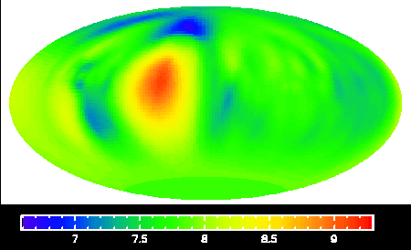
Just 1 line used with 106 points and 20 phases.
The spots to the right and to the left of the
central spot in Fig. 7 of S12 start to emerge.


K) 28.1.2012

"The unspecified “eccentric dipole” with an unusually high contrast
(field strength variation by a factor of 3.7 instead of a factor of
2 expected for a centred dipole) seems to have been hand-picked to
maximise profile differences."

Are we entitled to ask the authors since when the centred dipole
model has imposed itself as the only realistic description of the
magnetic geometry of Ap stars? Has not O. Kochukhov himself
repeatedly found strong quadrupole contributions in several Ap
stars (which as we know can be equivalent to a decentred dipole)?
Has the whole literature on decentred and sometimes tilted dipole
models not been available to the authors, including papers by
J. Landstreet and by M.J. Stift? And finally, concerning the
"hand-picking" of an allegedly "maximised difference", has not
O. Kochukhov himself found variations in field strength by a
factor of more than 6 (!!!) in 53 Cam?

"However, the scenario considered is not applicable to the case of
alpha2 CVn because the adopted spot diameter is underestimated by
a factor of two and the imposed correlation of the small-scale
abundance and magnetic field enhancements is contrary to what was
found for that star."

Is it again frivolous to ask why the authors so much insist on looking
exclusively at 1 star in their attempted refutation of the findings of
S12? Did they ever realise that the assumption of a spot of 50 deg
radius can have nothing to do with their favourite star, that the
discussion by S12 went further than a critique of the analysis of
1 star among many others? Would they subscribe to the opinion that
even the findings presented in Fig. 7 of S12 would apply to one and
only one star, by no means applicable to any other star in the
universe? Don't simulations and inversions based on a resolution of
R ~ 35000 and 20 phases also apply to another famous star, viz.
53 Cam? Did S12 not explicitly speak of an "inversion of a single
line as in Kochukhov et al. (2004)" but not "as in Kochukhov et al.
(2010)"? Was the emphasis not on ZDM in general instead of ZDM
applied to 1 single star when S12 mused: "It is not easy to assess
which of our findings will have the most sobering effect on (Zeeman)
Doppler mapping enthusiasts keen on claiming to have found small-scale
and high-contrast structure on the surfaces of magnetic Ap stars"?
And what again about the "correlation of the small-scale abundance
and magnetic field enhancements" which in the case of 53 Cam is more
or less exactly as S12 have assumed, with a field of more then 20kG
found in places where iron is extremely overabundant?

"Furthermore S12 produced a small-scale magnetic feature by
simply scaling all three vector components in an arbitrarily chosen
location on the star instead of introducing horizontal field structures
similar to those found for alpha2 CVn by KW10."

Who would be able to follow this argument? Doesn't scaling of all
3 vector components instead of scaling of just 1 component simply
give a larger signal over the rotation period both in linear and
in circular polarisation? Where is the problem, where a possible
bias against KW10?


L) 29.1.2012

"Our results convincingly demonstrate that the bleak S12 assessment of
this magnetic inversion procedure is grossly in error. It appears that
their allegations are based on an unreasonable extrapolation of a very
limited set of forward Stokes parameter calculations for an artificial
abundance distribution not resembling any real Ap star. The outcome of
the inversions proper, presented here, proves that the methodology
used by S12 is misleading and erroneous. A general conclusion, which
inevitably follows from this discussion, is that the S12 assertions are
largely irrelevant in the context of modern MDI studies by KW10,
Kochukhov et al. (2002, 2004a), and L¨uftinger et al. (2010b)."

Isn't it remarkable that it should follow "inevitably" from the
discussion of just 1 star, viz. alpha2 CVn, that the effects found
and discussed by S12 should be "largely irrelevant" to other stars?
Has it really been shown beyond reasonable doubt (or even at all) in
KW10 that the extreme field values around the visible pole of 53 Cam
do not affect the Fe abundances derived without taking into account
the local atmosphere? Has it ever been discussed in some way, let
alone quantified, in KW10 (or even better in Kochukhov et al. 2004)
how the vast Fe overabundances would affect the Stokes IQUV profiles
of 53 Cam? Isn't it true that the various spots, near the pole and
at moderate latitudes, cover far more than a mere 1-2% of the stellar
hemisphere? Would the authors deny that the strong Fe II 4923.93
spot visible in Fig. 6 of Kochukhov et al. (2004) -- strangely almost
completely absent in Fe II 5018.44 and significantly displaced in
Fe II 5169.03 -- is associated with a field of more than 10kG
strength? Do the maps for individual lines in Fig. 6 not agree that
near the pole the field strength exceeds 20kG with the iron abundance
reaching [Fe] = -2.0 over a sizeable fraction of the polar cap?
Have the authors ever given the guarantee that the sometimes huge
gradients found around the spots of 53 Cam (depending on the line
used, the differences range from 1 to 3 dex for exactly the same <- corrected
region on the star) are not artefacts of their inversion similar
to those presented by S12 in their Fig. 8 ?

Does it add to the credibility of the strong statement cited above
that a minuscule Fe II 4923.93 abundance spot not only disappears but
changes sign in Fe II 5169.03 ? Inexplicably and unexplainedly, a point
exhibiting [Fe]= -3.0 in one line becomes a point with [Fe] = -5.0 or
even less in another line. A conspicuous and, as we are told in the
context of alpha2 CVn, necessarily significant point of higher abundance
in some region becomes a less conspicuous, but still necessarily
significant point of lower abundance.

Isn't the judgement made by the authors and cited above rather severe
but not overly coherent? If an assessment is "grossly in error", if
everything is based on "unreasonable extrapolations", if "the methodology
is misleading and erroneous" (note the exquisitely restrained prose!),
isn't it a pleasant albeit somewhat bewildering surprise to read that
the S12 assertions are merely "largely irrelevant" but do not have to be
completely discarded? Isn't it great that this partial irrelevance of
the S12 findings is restricted to exactly 4 "modern" studies (it is clear
that the authors do not write "such as KW10 ..." for good reasons of
their own), leaving all the other less "modern" papers open to the
well-founded S12 criticism?


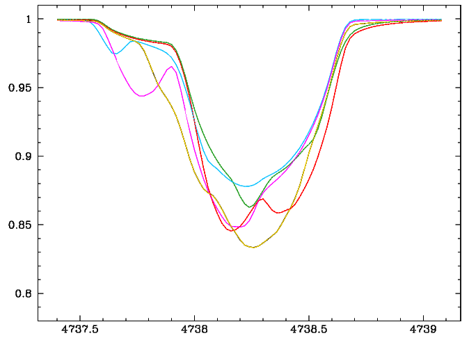
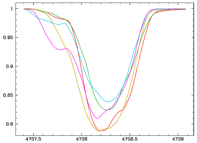
M) 30.1.2012

Isn't there magic in the air? Who would have thought that an "untested"
inversion code with "serious problems" would miraculously (albeit for
some people not surprisingly) manage to recover remarkably well the
input data to Fig. 7 of S12 ? Would you believe that neither input
physics nor algorithms have changed since S12, and that a few minor
modifications to the CossamDoppler code have resulted in a speedup of
between a factor of 10 and 50 ? Aren't our 2 figures a convincing
demonstration of the dangers inherent in single-line inversions as
presented by Kochukhov et al. (2004)? May we ask in the light of
these results how reliable are the extremely high abundances near
the pole of 53 Cam prominently visible at phase 0.40 in Fe II
4923.93 but largely absent in Fe II 5169.03 and turning into an
underabundance spot in Fe II 5018.44 ? Isn't it distressing to see
so much fine structure in Fig. 6 of Kochukhov et al. (2004) go from
black to white and vice versa, depending on the Fe II line used?



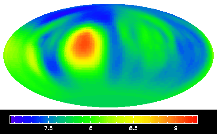
3 lines used with 144 points and 20 phases.
The spots to the right and to the left of the
central spot in Fig. 7 of S12 (and their structure)
are now clearly visible. Based on "usual" profiles
and "usual" inversion.



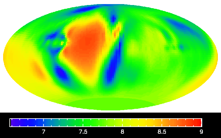
3 lines used with 144 points and 20 phases.
Based on "correct" profiles and "usual" inversion.
Who would insist that the effects of metallicity
on the local atmosphere are "largely irrelevant in
the context of modern MDI studies"?

Is it not alarming that the differences between the 2 maps range
between -1.15 dex and +0.85 dex, resulting in a staggering 2 dex
amplitude in the difference map? Is it not deeply disturbing
that a mere 1.5 dex maximum contrast in the original map changes
to about 2.5 dex in the map obtained with the "usual" inversion
applied to the "correct" profiles?


N) 31.1.2012

Aren't we living in wonderful times full of exciting discoveries?
Don't observers flood us with the finest spectra, analysed in the
most sophisticated way, and yielding the most surprising results?
And don't these results, figure by figure, line by line, abundance
by abundance, demonstrate how necessary it was for the authors to
point out all the alleged shortcomings of S12?

Would you consider it strange that the authors did not cite a paper
by Nesvacil et al. (2012) in their huge bibliography, despite D.
Shulyak and O. Kochukhov being co-authors? Isn't it disappointing
to see that they did not confront the findings of this paper with
the main points of criticism towards S12 to further bring home their
arguments? Let me try to do this work for the authors, but modesty
of course does not permit me to pretend that it could ever be
as clear, profound or considerate as is typical for the authors.

1) "The choice by S12 of the abundance DI studies yielding “unrealistic”
elemental overabundances is highly selective, confined to two extreme
results, both published in conference proceedings (Kuschnig et al.
1998; Piskunov et al. 1998). This ignores the majority of DI studies
published in the refereed literature which reported much more modest
abundance contrasts."
Aren't we now at last in the presence of a refereed paper, but with
abundances even more extreme than those found in the cited papers?
Do we not have to congratulate N. Piskunov for the discovery of a
star without any hydrogen (nor He or CNO or Fe or Ca ...) in parts
of its atmosphere, 14 years after "conference proceedings" that
announced an A&A paper on a new kind of Cr star which however never
appeared? With the wonderful spots in Figs. 4-6 of Nesvacil staring
at us, aren't we entitled to have a close look at extreme results
including this fascinating article?

2)"In the actual Fe map published by KW10 only 2.5% of the visible
surface has logNFe/Ntot > −2."
Could it be that in HD3980 we are now not only faced with spots and
rings of extreme iron abundances, but also of huge oxygen, manganese,
silicon, calcium and chromium over-abundances? Would the authors
claim that a spot of uncannily high abundance of oxygen and of
manganese that takes up ~15% or more of the visible surface would
be negligible in the analysis, especially when you take into account
the extended bands of Ca, Cr, and Fe which run over this spot? And
should one really forget the magnetic field which allegedly reaches
its maximum in this spot?

3) "But this profoundly multi-line, multi-phase character of modern
MDI was not considered by S12, who limited their analysis to a
single spectral line at one rotational phase."
Who would not adore a genuine multi-line DI or MDI analysis? But
looking again at Nesvacil et al. (2012) is there much "multi" to be
seen? Is it not true that the Eu, Ca, Pr, and Nd maps are based on
just 1 line. That the Mn, Gd, Fe, and Si maps are derived from a
mere 2 lines? So why should S12 not have had a look at single-line
analyses which actually pervade (M)DI from Kochukhov et al. (2004)
and earlier up to the present day? Turning to the "multi-phase"
character, has the Mn map not been derived from only 12 phases?

4) "Thus, the lack of very high elemental overabundances in the
equilibrium diffusion calculations is an artefact of the limited
computational capabilities of the currently used atomic diffusion
codes."
"No obvious correlation between theoretical predictions of diffusion
in CP stars and the abundance patterns could be found. This is
likely attributed to a lack of up-to-date theoretical models."

From where do O. Kochukhov and D. Shulyak take their conviction that
their results can constitute a "challenge" to diffusion theory? Why do
they think that there is a lack of up-to-date theoretical models when
a warped analysis -- that does not even take into account the magnetic
field -- yields frighteningly weird abundances and exceedingly poor
fits to many spectral lines over many phases? What about synthetic
profiles that differ by up to 2% from the observed profiles, often
with large systematic deviations from the wings to the core? Can these
inversions be considered up-to-date, correct or even just credible?

Isn't the lack of models that explain the strange maps in Piskunov et
al. (1998) -- more Cr than H -- or in Nesvacil et al. (2012) -- just
Si and no H -- simply a healthy sign of a sane diffusion theory?


O) 01.02.2012

"In the present Doppler imaging analysis we used a nonmagnetic
spectrum synthesis for computating (sic!) the line profiles of
respective elements."
"We found that including the Zeeman splitting in the presence of a
magnetic field leads to an abundance decrease of 0.10−0.15 dex for
Fe and Cr."
"Except for Eu and Gd, the upper abundance limits of the maps
computed with INVERS12 are not very affected by neglecting the
magnetic field. Lower abundance limits are not influenced as much
for any of the lines used for mapping."

When O. Kochukhov and D. Shulyak make these statements in Nesvacil
et al. (2012) (Nes12) is one not entitled to ask what happens to
the abundances of other elements than Fe, Cr, Eu and Gd? What about
the phenomenal Si spots, 2 of which largely coincide in position
with the poles of the magnetic field? What about oxygen and
manganese with conspicuous spots exactly around the magnetic
poles? Is the effect on abundance of Zeeman splitting really our
only concern? Wouldn't profiles of both incredibly and reasonably
abundant elements not only display large magnetic intensifications
but more importantly exhibit local profiles completely at variance
with non-magnetic profiles? What about Doppler mapping using such
blatantly incorrect profiles, can it be expected to yield correct
maps? Where are the tests to prove such an unlikely scenario?



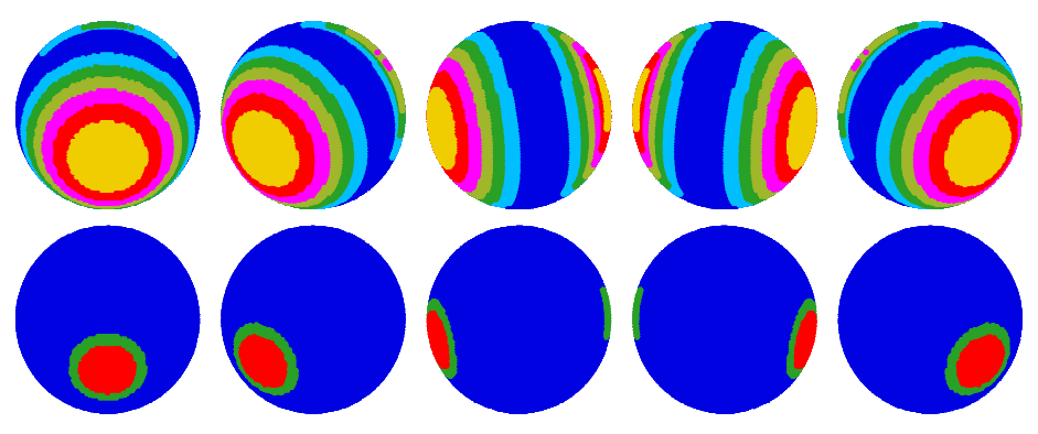
It is not difficult to simulate the difference between a magnetic
and a non-magnetic profile of the Mn lines used by Nes12. This
plot shows the positions of 2 manganese spots at different phases
(lower panel). Blue corresponds to [Mn] = -4.50, green to -3.0
and red to -2.0 (am I not right, even for tests, not to exaggerate
or to indulge in unwarranted extremes and/or extrapolations?). The
magnetic field strength of the centred dipole is presented in the
upper panel and corresponds to the values claimed by Nes12. Sizes
and positions of the spots are not unlike those found in Fig. 4
of Nes12; maybe they are slightly too small.




Would Kochukhov and Shulyak agree that even in the integrated
case the non-magnetic profiles (above) differ consistently and
quite substantially from the magnetic profiles (below)? In the
light of these profiles, can anyone genuinely expect that their
Mn maps of HD3980 reflect true geometry and at least approximate
abundances?




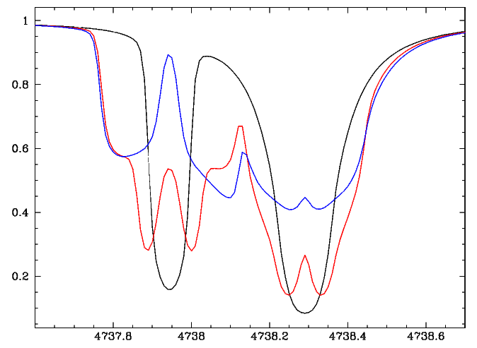
Wouldn't these findings make it desirable to have a close
look at what actually happens to the local Mn profile at
the magnetic pole? Isn't this something that Kochukhov
and Shulyak unexplicably fail to provide. Never mind,
aren't there free Stokes codes available to check? Once
you have carried out the straightforward calculations, can
you detect anything in common between the non-magnetic
profile (black), the magnetic profile in the longitudinal
case (blue) and in the transversal case (red)? Can the
authors ever reassure us that these huge differences in
shape will not create unsurmountable problems when Doppler
mapping of a strongly magnetic star is carried out with
non-magnetic profiles?





P) 02.02.2012

Isn't it fascinating, revealing and worrisome, all at the same
time, to see yet another example of how abundance maps can change
with time and authors, to find no explanation on how this can
possibly happen, and one all-pervading constant: O. Kochukhov
invariably being co-author? Haven't Obbrugger et al. (2012) (Ob12)
used INVERS12, LL models and Synth3 for their Li, Pr, Gd, Fe, and
Cr maps of HD3980? Did they not announce "The next steps will
include the investigation of more lines to improve the determined
abundance patterns" and didn't they fail on this promise for at
least 4 out of 5 elements? Do we not see, 4 years and the same
number of lines later, Fe and Cr abundances both range between
-5.3 and -2.3, whereas they previously went from -6.0 to -1.5 and
from -7.0 to -1.5 respectively? Did the Li blend in not indicate
abundances ranging from -9.5 to -2.5 in 2008, -10.0 to -4.0 in
2012, consistently derived without taking into account the magnetic
field, not to speak of the Paschen-Back effect?

Would it again be frivolous to ask what may cause the Pr spot --
based on a single line -- to expand, and why the 2008 patterns
of the other elements are sometimes distorted almost beyond
recognition in the 2012 maps? Is it due to additional observations
or is it an artefact of observations omitted in the 2012 analysis?
Isn't it strange and thought-provoking that phases 0.498, 0.499,
0.515, 0.642, 0.643 (to name a few) no longer show up in Nes12 ?
Are the new fits to Fe 6065.48 and Fe 6230.74 at phases 0.827,
0.959, 0.020, and 0.023 in Nes12 any better because they now lie
above the observed profiles instead of lying below as in Ob12 ?

"It is known that the formation of the Li i 6707.473 Å line is
subject to the Paschen-Back effect (see Kochukhov 2008a; Stift
et al. 2008), which becomes noticeable around 3 kG. However,
we did not account for this in the present study because
a) modeling the Paschen-Back effect is a non-trivial task that
requires special software and complex techniques;
b) the true geometry of the global magnetic field of HD 3980 is
not known, i.e. its deviation from the simple dipole would
introduce additional uncertainties in the line profile fitting
with magnetic spectrum synthesis; and
c) the star’s rather high v sin i = 22.5 kms−1 smears out the
line profile shape considerably."

Do these arguments not leave us stunned and breathless? Has not
Kochukhov (2008) presented a paper on the Paschen-Back effect in
Li, boasting: "Other important point is that all previous studies
of PB effect in magnetic stars were purely theoretical. My paper
is the first to apply these calculations to a real astrophysical
problem and to confront theoretical spectra with actual stellar
observations"? So why has this "special software" mentioned in
this article not been applied, why has the "non-trivial task"
not been undertaken, why have the "complex techniques" not been
refined even further?

Does O. Kochukhov really want us to believe that disregarding
the magnetic field completely would yield more reliable results
than a magnetic analysis (with or without PB) with a rough
estimate of the magnetic field geometry? Is it not rather
true that he lacks the "special software" necessary for a proper
PB analysis, that it would be inappropriate to speak of a PB
code of his in the same sense as of the INVERS12 code? Are people
completely off the track when they surmise that the PB approach
by Kochukhov is working only for an extremely restricted set of
very special (symmetric) magnetic geometries?


Q) 03.02.2012

"A subsequent study by Kochukhov & Piskunov (2002, hereafter
KP02) presented extensive numerical experiments designed to
evaluate performance of INVERS10. These tests demonstrated that,
given high-resolution IQUV observations, the magnetic inversion
code is capable of correctly reconstructing abundance and
magnetic field vector surface distributions simultaneously and
without any prior assumptions about the large-scale magnetic
field geometry.

In the original Kochukhov & Piskunov (2002) paper we read:

"We have chosen the rotational velocity v sin i = 30 kms−1
and inclination angle i = 60 deg, which are optimal for DI.
In addition, modelling linear polarization profiles requires
specifying the angle theta (0 deg <= theta <= 360 deg)
between the stellar rotational axis and the local meridian
projected on the sky. We used theta = 90 deg throughout
this paper."

"For the evaluation of the disk-integrated Stokes parameters
we employed a spatial grid divided into 695 surface zones.
This grid size proved to be adequate for the calculation of
the Stokes flux profiles for the adopted value of v sin i ..."

"The reference magnetic topology of our DI tests consisted of
a dipole with polar strength Bd = 8 kG, positioned in the
plane of the stellar rotational equator, and with the positive
magnetic pole crossing the plane containing the line-of-sight
and the stellar rotational axis at zero phase ... Such a
magnetic geometry, rotational velocity and inclination
collaborate to maximize the magnetic variability of the
spectral line profiles and represent an ideal combination
for the application of MDI."

"All Stokes profiles in this paper were calculated for the
iron doublet Fe II 6147.74 A and 6149.26 A."

"The Fe II 6147.74 A and 6149.26 A spectral lines are known to
have different magnetic sensitivities and serve as a primary
spectral diagnostic for the surface field modulus of slowly
rotating Ap stars."

"We used an iron abundance eps(Fe) = log (N_Fe/N_total) = −4.0
outside spots and eps(Fe) = −2.5 inside iron concentrations."

"Synthetic observational data were simulated for 10 equidistant
rotational phases and convolved with the Gaussian instrumental
profile with FWHM = 61 mA (corresponding to the spectral
resolution R = 100 000 at lambda = 6148 A). Random noise with
an amplitude of sigma_I = 3.3 10^-3 (S=N = 300) was added to
Stokes I profiles, while noise levels in Stokes V and Stokes QU
were scaled down by a factor of 1.5 and 4, respectively."

Now, do for example Kochukhov et al. (2004) and Kochukhov & Wade
(2010) not base their analyses on spectra with only R = 35000?
Is it not equally true that only 2 out of 19 spectra of 53 Cam
exhibit a peak S/N of 300 and better?

How do we have to understand the "extensive tests"? Do we have
to consider them realistic or have they rather been designed,
by admission of Kochukhov & Piskunov (KP02) themselves, to be
based on rotational velocities and angles "which are optimal
for DI"? Did KP02 not explicitly state that "magnetic geometry,
rotational velocity and inclination collaborate to maximize
the magnetic variability"? Was the choice of the 2 Fe lines not
also made because of their "different magnetic sensitivities?
How could a correctly written inversion code possibly fail to
converge to the highly artificial input map consisting of a small
number of symmetric high-contrast spots in a simple geometric
arrangement, when optimum parameters for DI have been chosen and
the magnetic variability maximised?

S12 had a look at what happens when parameters do not combine as
ideally as in the KP02 tests; the figures under J) and M) reveal
that smooth maps are no guarantee to correct results. Where is the
much desired and required paper by Kochukhov that would present
tests for less favourable abundance geometries, more modest field
strengths, and realistic spectral resolutions?

  Back to the Ada in Astrophysics Homepage